# Simple example of regression discontinuity design
set.seed(42)
n = 1000; threshold = 0
X = runif(n, -1, 1)
W = as.numeric(X >= threshold)
Y = (1 + 2*W)*(1 + X^2) + 1 / (1 + exp(X)) + rnorm(n, sd = .5)
out = plrd(Y, X, threshold)
print(out)
#> Partially linear regression discontinuity inference:
#> Threshold: 0
#> Lipschitz constant: 7.302
#> Max bias: 0.05186
#> Sampling SE: 0.0856
#> Effective sample size: 990
#> Confidence level: 95%
#>
#>             Estimate CI Lower CI Upper    p-value
#> RD Estimate    2.022    1.828    2.217 1.461e-117
# default plot: scatterplot of original data with black curves showing
# representative regression functions in our data-driven function class
plot(out)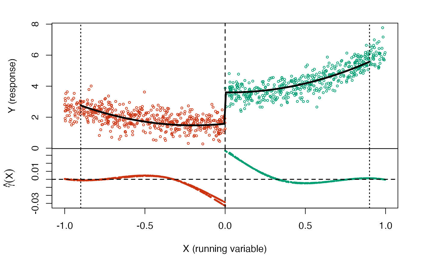
# plot of plrd weights (two sets of weights because we use cross-fitting)
plot(out, type = "weights")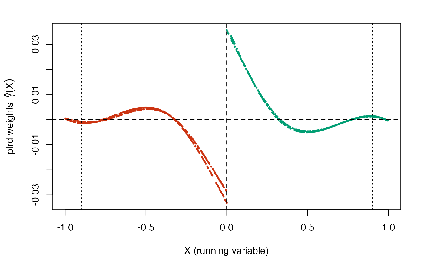
# fancy plot option that combines the previous two plots
plot(out, type = "combined")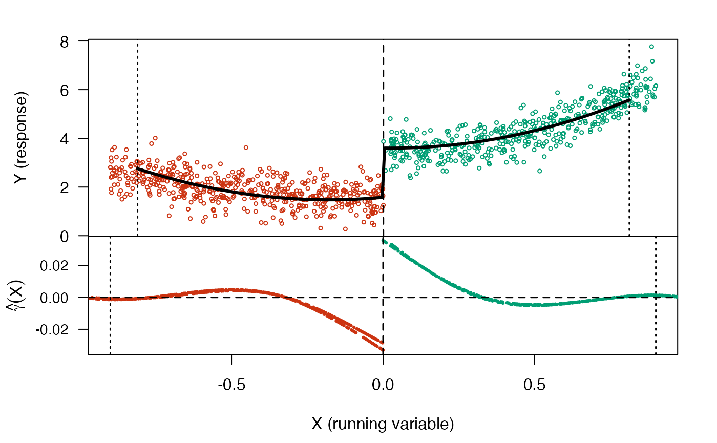
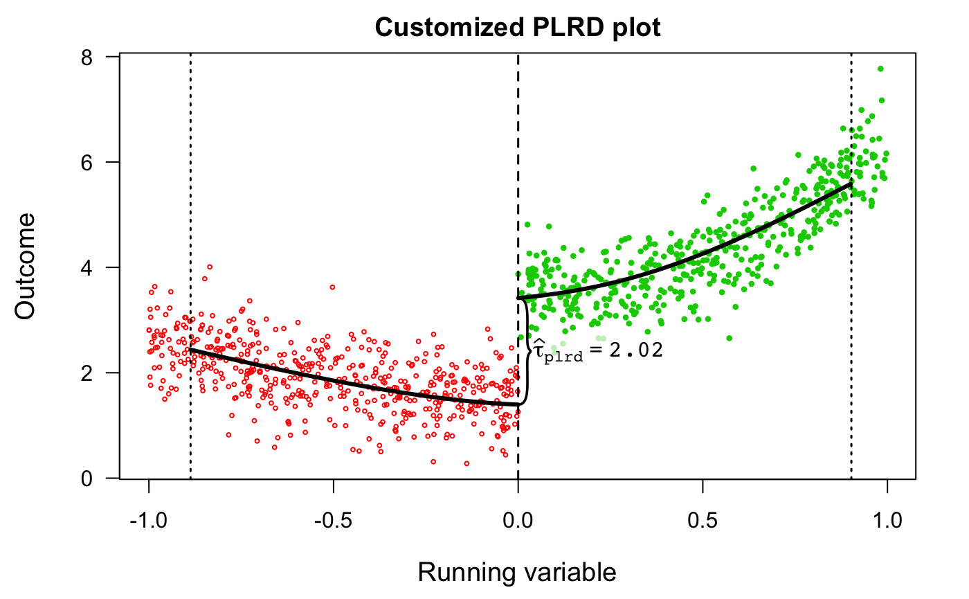
The plotting method accepts standard graphical arguments for further customization.
plot(
  out,
  main = "Customized PLRD plot",
  xlab = "Running variable",
  ylab = "Outcome",
  annotate.tau = TRUE,
  las = 1,
  cex.lab = 1.2,
  col = c("red", "green3", "black"),
  pch = c(1, 16),
  cex = c(.4, .6)
)